Is learning R hard for SAS users, absolutely not !!

I am an avid R user and rarely use anything else for data analysis and visualisations. While R is my go-to, in some cases, I use Python too. But, I have switched from SAS which I used for over 6 years. A data guy needs to keep his tools sharp all the time. SAS has been promiment choice but R and Python catching up fast.
SAS users sometime hesistate to learn R because its perceived as “complex programming language”. That’s why I wanted to demonstrate how R and SAS fare in a one-on-one comparison on basic analyses that’s representative of what an analyst would typically work with. Just to get the feeler, let’s see through some examples that how does R and SAS do some basic stuff.
The idea of this write-up is not to compare the two but to highlight the similarity so that a SAS user can easily grasp R when need arises. I am listing down easy to do thing in R and SAS.
Conclusions
All in all, the SAS code could easily be translated into R and was comparable in length and simplicity between the two languages. While R’s syntax is inherently cleaner/ tidier, we can always use packages that implement similar function as in SAS and achieve similar results. For plotting and visualisation I still think that R’s ggplot2 is top of the line in both syntax, customizability and outcome (admittedly, I don’t know SAS/GRAPH too well !). In terms of functionality, I couldn’t find major differences between the two languages and I would say they both have their merits. For me, R comes more natural as that is what I’m more fluent in, but I can see why SAS holds an appeal too. In my perspective that there is lot of similarity between SAS and R and it is not hard to switch onto R from SAS. Although, they both have pros and cons and in short term future they both need to co-exist. So, using both technologies to leverage data manipulation and data analysis seems like the winning solution for all.
So , let’s get started and for the things that you don’t know, GOOGLE is always there ![]() .
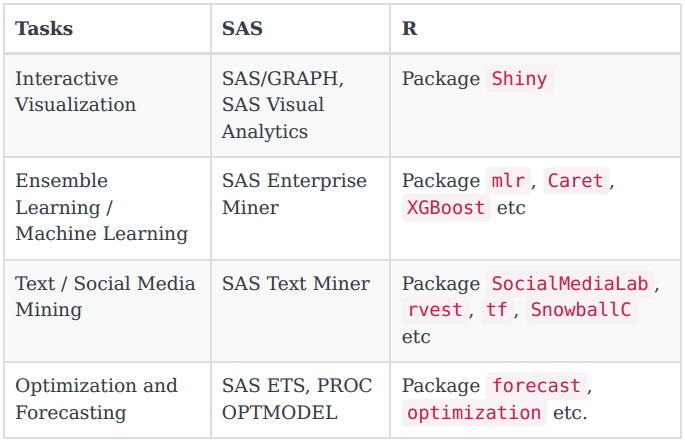
First of all, let’s see what R have in parallel with SAS functionality:
.
First of all, let’s see what R have in parallel with SAS functionality:
For R, I am working with RStudio. You can install R Studio from here. It enables you to see your codes, execute them, see output and manage the project. R studio looks like this :
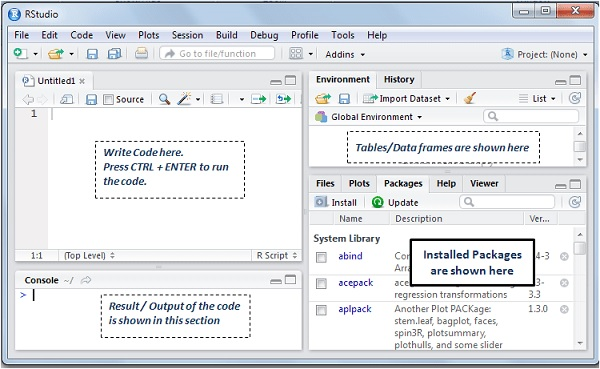
So you write code in the upper left ( editor pane) and hit ctrl + enter so see the new datasets or other objects in Environment tab in upper right pane. for SAS I am refering to Base SAS 9.4.. I am assuming you have Base SAS , so open SAS editor and see how does these codes work.
Small notes
- In SAS, we refer data files as datasets and in R we refer them as dataframes.
- In R, we use forward slash for path reference. E.g SAS path is referenced as “C:\My_Project\file.txt” but in R “C:/My_Project/file.txt”.
Let’s see does these two work for some basic data manipulation tasks:
- Import data
- Export data
- Select observation
- Select variables
- Transform variables
- Conditional transformations
- Renaming variables
- Stacking or concatenating data
- Joining or merging data
- Basic data analysis
In both SAS and R, a task can be performed by various ways. For example, for importing data, one can use PROC import or INFILE statement in SAS. For sake of ease I am using the simpler way of performing a task.
Import data
So what is the first thing we do in any anlaytics projects , import data - right ? Let’s do it. Of course, you need to have a csv file names as “mydata.csv” on your computer.
SAS
PROC IMPORT DATAFILE="D:\mydata.csv"
     OUT=MYDATA DBMS=CSV REPLACE;
     GETNAMES=NO;
RUN;
R
data<- read.csv("D:/mydata.csv")
See, I used forward slash in R, while mentioning folder path. You’ll see a dataframe named “df” in Environment tab in upper right pane on RStudio.
Export data
Export is not much different either, few keywords here and there in the syntax and boom !!
SAS
PROC EXPORT DATA=SASHELP.CLASS
     OUTFILE='C:\TEMP\SASHELP mydata.csv'
     DBMS=CSV
     REPLACE;
RUN;
R
write.csv(data, "D:/mydata_export.csv")
In R, you can write data in various formats, you can export in .sas7bdat format as well, check out write.table() and write.foreign() functions.
Select observation
Let’s say, I want to filter data based on column of data, I’d use:
SAS
DATA SASUSER.FEMALES;
     SET SASUSER.MYDATA;
     WHERE GENDER="F";
RUN;
R
female_data<- mydata[mydata$GENDER=="F", ]
In SAS, to select observation, we also use logical conditions with commands like IF, WHERE or SELECT IF. In R, mydata is structured as mydata[row,column] matrix, so you can play around by directly apply logical condition to “rows” and “columns” at the same time . Try something like below in R:
FEMALES<- mydata[mydata$GENDER=="F",c(1:3)]
Select variables
Selecting variables in SAS is quite simple, it can be easily done through KEEP or DROP keyword at data step.
SAS
DATA MYDATA;
     SET MYDATA;
     KEEP AGE GENDER;
RUN;
Well, in R its not that difficult too.
R
mydata<- mydata[ ,c("AGE","INCOME")]
In R, columns can be referred in various ways:
By name : As you have seen above in the code. I am asking R to produce columns that has “AGE” or “GENDER” as column name.
By index number : mydata[3] is almost the same as mydata[ ,3] -both refer to third variable of the dataframe mydata.
By index number sequence : mydata[3:6] is almost the same as mydata[ ,3:6] -both refer to third , fourth fifth and sixth variable of the dataframe mydata.
By logical vectors : For example, mydata[,c(FALSE,FALSE,TRUE)] will select the third column only because the 3rd value is TRUE.
Transform variables
Unlike SAS, R has no separation of phases like the data step and proc steps. In fact, you can even modify variables in the middle of procedures as shown in example below.
SAS
DATA SASUSER.MYDATA;
    SET  SASUSER.MYDATA;
    TOTAL_MARKS=(MARKS_1+MARKS_2+MARKS_3);
LOG_TOTAL_MARKS=LOG10(TOTAL_MARKS);
RUN;
R
mydata$TOTAL_MARKS<- mydata$MARKS_1 + mydata$MARKS_2 + mydata$MARKS_3
mydata$LOG_TOTAL_MARKS<- LOG(mydata$TOTAL_MARKS)
Conditional transformations
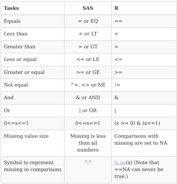
Through conditional transformations we apply different formulas to various subgroups of the data. Below are the logical operators for SAS and R and how a few comparisons differ or match.
The examples below demonstrate a rather complex conditional transformations.
SAS
DATA SASUSER.mydata;
  SET SASUSER.mydata;
IF MARKS_1>  75 & MARKS_2 > 75 & MARKS_3 > 75 THEN GRADE="DISTINCTION"; ELSE GRADE="NON-DISTINCTION";
RUN;
R
myadata$GRADE <- ifelse( mydata$MARKS_1 >75 & mydat$MARKS_1 >75 & mydata$MARKS_1>75,"DISTINCTION","NON-DISTINCTION" )
So, you can create and transform variable based on other columns, in one go.
Renaming variables
In R, however, both row and column names are stored in character vectors within the data frame. In essence, they are just another form of variable that you can manipulate. In R , names() is the vector that stores the columns header so we can use to change name of the columns.
SAS
DATA SASUSER.mydata;
  RENAME q1-q4=x1-x4;
RUN;
R
mydata <- rename(mydata, c(MARKS_1="MARKS_MATHS"))
R has reshape () package, that offers similar approach for renaming variable as SAS. Example,
R
library(reshape)
mydata <- rename(mydata, c(q2="x2"))
Stacking or concatenating data
Very often, we land into scenario where you have to join a data to another data. It this example we’ll see how to put together two datasets spitted from same file. In SAS , it’s called setting or appending, in R it’s called binding rows.
SAS
DATA DISTINCTION   ; SET mydata; WHERE GRADE="DISTINCTION"; RUN;
DATA NON_DISTINCTION ; SET mydata; WHERE GRADE="NON-DISTINCTION"; RUN;
DATA BOTH;    SET MALES FEMALES;  RUN;
R
distinction_data <- mydata[mydata$GRADE=="DISTINCTION", ]
non_distinstion_data <- mydata[mydata$GRADE=="NON-DISTINCTION", ]
both <-rbind(distinction,non_distinction)
In R, you can bind columns too, try cbind().
Joining or merging data
Joining and merging is one of the frequently used data operation that you’ll be doing. Let’s see through an example how does R do it. Let’s create two datasets selecting some variables from a big dataset. My base dataset “MYDATA” has 5 variables - “ID”,” MARKS_1”,” MARKS_2”,” MARKS_3”,” MARKS_4”. I split the data with three variables each.
SAS
DATA myleft; SET MYDATA; KEEP ID GENDER MARKS_1 MARKS_2; PROC SORT; BY ID; RUN;
DATA myleft; SET MYDATA; KEEP ID NAMES  MARKS_3 MARKS_4; PROC SORT; BY ID; RUN;

DATA BOTH; MERGE MYLEFT MYRIGHT; BY ID ; RUN;
R
myleft<-mydata[ ,c("ID","GENDER","MARKS_1","MARKS_2") ]
myright<-mydata[ ,c("ID","NAMES","MARKS_3","MARKS_4") ]

both<-merge(myleft,myright,by="ID")
Basic data analysis
In this section, let ‘see some very basic hypothesis tests done in SAS as well as R.
Let’s pretend we have a dataset “mydata.csv” with 4 numeric variables V1 , V2, V3 and V4.
Let see how can we perform some basic data analysis to know the profile of data elements using SAS and R.
SAS
               /** BASIC STATS **/

/* BASIC STATS IN COMPACT FORM*/
PROC MEANS; VAR V1-V4; RUN;

/* BASIC STATS OF EVERY SORT */
 PROC UNIVARIATE; VAR V1-V4; RUN;

/* FREQUENCIES & PERCENTS*/
PROC FREQ; TABLES V1-V4; RUN;

              /** CORRELATION **/

/* PEARSON CORRELATIONS */
PROC CORR; VAR V1-V4; RUN;

/* SPEARMAN CORRELATIONS*/
PROC CORR SPEARMAN; VAR Q1-Q4; RUN
R
library(foreign)
library(Hmisc)
library(prettyR)
# Descriptive stats and frequencies.
summary(mydata)

# Means, freqencies & percents
describe(mydata)

# Frequencies & percents
freq(mydata)

# Pearson correlations.
cor(data.frame(q1,q2,q3,q4),method="pearson")

# Spearman correlations.
cor(data.frame(q1,q2,q3,q4),method="pearson")
I am intentionally not touching upon other measure of association such as group comparisons and t-test and Chi-square test which involves categorical variables and some more knowledge of probability and distribution. You can always refer to Hmisc() package for more coverage.