Last few days I have been working on a images classification challenge and I have been reading papers on density based clustering.

The basic goal of clustering is to find groups of data points that are similar to each other. Also, data points in one group should be dissimilar to data in other clusters.

Before we go there let me explain the difference between k-mean based clsutering and density based clustering .

K-means clustering aims to partition n observations into k clusters in which each observation belongs to the cluster with the nearest mean.

Density-based clustering algorithm finds a number of clusters starting from the estimated density distribution of corresponding nodes.

In simple words, K-means just looks for the proximity of other points whereas Density-Based Spatial Clustering of Applications with Noise (DBSCAN) also takes care density and noise in a cluster before assigning a cluster .

The advantages of DBSCAN are:

- Unlike K-means, DBSCAN does not require the user to specify the number of clusters to be generated
- DBSCAN can find any shape of clusters. The cluster doesn’t have to be circular.
- DBSCAN can identify outliers

As image is data in matrix shape and density of pixels have to be compared in order to find closer one so , I have chosen DBSCAN over k- means to cluster the pictures.

I have used the NOAA data for fishes published for a fish recognition competetion. It’s public data and available here.

There are 3777 pictures and I wanted to identfy if some of these pictures are similar because they are of same boat.

The motivation for me was, if I can group picture by their similarity , then this group identifier can give me some boost on leaderboard.It so happened that I coudn’t submit my final score because of some last minutes changes in my schedule.

But none the less , it gave me idea to apply this algorithm to group the similar pictures.

Let’s save the pictures to a local directory and begin with this.

# Loading libraries

library(data.table)
library(gtools)
library(fpc)
library(dbscan)
library(factoextra)
library(imager)

# This function will randomize the list and pick sample pictures and converts them into dataframe, one row for one pic, modelling on all may  take super long

random_pic_selection<- function(folderpath, samp, res) {
  std_data= list()
  df= data.frame()
  piclist<- sample((list.files(folderpath, pattern=".jpg", full.names=TRUE, recursive = T)) 
                   , ((samp/100)* length(list.files(folderpath, pattern=".jpg", full.names=TRUE, recursive = T
                   ) )))

for (i in 1:length(piclist)) {
    
    im<- load.image(piclist[i]) # read image
    im_res <- resize(im, res, res)  # resizing image 
    im_std<-(im_res-mean(im_res))/sd(im_res) # standardizing image 
    img_std_data <- as.data.frame(im_std)
    img_std_vector <- as.vector(img_std_data$value)
    img_name<-paste0(basename(piclist[i]))
    vec_std <- c(img_name=img_name,img_std_vector)
    std_data[[i]]<-vec_std
    
    print(paste0( "Pic - ",i , " successfully converted ", piclist[i]))
  }
  
  df<- as.data.frame(do.call(rbind, std_data))
  return(df)
  
}

If we call the above function , we’ll get image converted as dataframe. We can choose the resolution of the pictures in res . I have kept resolution as 128 pixels to try and train the model. It creating 49152 columns , 128 rows X 128 colums X 3 color frames RGB = 49152.

Creating training and test dataset

I have chosen 10 % of 3777 pictures to train the model so , I gave samp = 10, this will get ~377 rows in train data frame.

folderpath = <c:/images/>
folderpath = "C:/R_RnD/Image_Segmentation/images/"
#Coverting data into numeric 
train_data<- random_pic_selection(folderpath , samp= 10, res=128)

The function DBSCAN digest input as numeric matrix , so I converted the data into numeric matrix.

# Converting train to numeric matrix
train_matrix<- as.matrix(train_data[,-1])
mode(train_matrix) = "numeric"

In this example, we’ll use dbscan package. A simplified format of the function is:

dbscan(data, eps, MinPts = 5, scale = FALSE, 
       method = c("hybrid", "raw", "dist"))

- data : data matrix, data frame or dissimilarity matrix (dist-object). Specify method = “dist” if the data should be interpreted as dissimilarity matrix or object. Otherwise Euclidean distances will be used.
- eps : Reachability maximum distance
- MinPts : Reachability minimum number of points
- scale : If TRUE, the data will be scaled
- method : Possible values are:
  - dist : Treats the data as distance matrix
  - raw : Treats the data as raw data
  - hybrid : Expect also raw data, but calculates partial distance matrices

The optimal value of “eps” parameter can be determined as follow:

k=kNNdistplot(train_matrix, k = 2)
abline(h = 160, lty = 2)

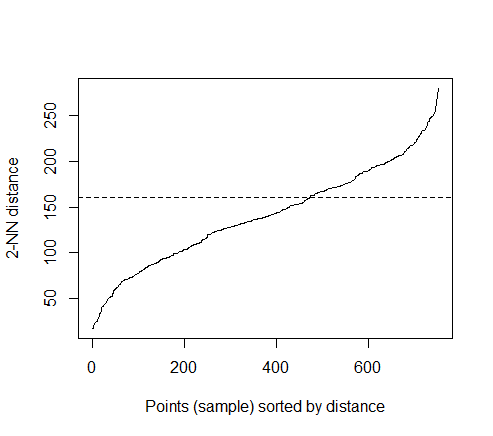
The thumb rule to find eps is to find the sudden uplift ( or knee) in NN distance. After trial and error , I found eps = 160 as good value to accept.

And, I chose MinPts=4 , meaning I expect at least 4 point in a cluster. Rest of the parameter are optional so I am letting them be default.

set.seed(1234)
dbscan_model <- dbscan::dbscan(train_matrix, eps = 160, minPts =4)

I have chosen dbscan algorithm of dbscan package because its faster implementation and I have large number of images to be segmented. dbscan from fpc package provide same result but its a bit slower.

Let’s check the final number of clusters

#  number of final cluster before drawing cluster map
table(dbscan_model$cluster)

  0   1   2   3   4   5   6   7   8   9  10  11  12  13  14  15  16 
200   7  63   8   4  14   9   4  24   4   4   7   5   7   8   5   4 

So, got 16 clusters, all the zeros are points that are not assigned any cluster. You may get slightly higher or lower number of clusters because of randomization of seed value.

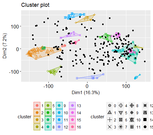
Plotting the results

The result can be visualized as follow:

fviz_cluster(dbscan_model, train_matrix, geom = "point")

Evaluation of clustering

# deriving names of image
evaluation_data_1<- data.frame(img_name=train_data[,1]) 

# assigning cluster to image
evaluation_data_1$cluster<- dbscan_model$cluster

#  selecting 4 images of a cluster in  dataframe
evaluation_data_2<-setorder(setDT(evaluation_data_1), cluster)[, head(.SD, 4), keyby = cluster]

# Sorting by cluster number for plotting purpose
evaluation_data_2<-evaluation_data_2[order(-cluster),] 

# changing to matrix for cell reference in below loop
evaluation_data_2<- as.matrix(evaluation_data_2)

#  plotting 4 images of 3 clusters
par(mfrow=c(2,2))
for (i in 1:12) {
plot(load.image(paste0(folderpath,evaluation_data_2[i,2])), main = paste0("Clus# ",evaluation_data_2[i,1]," \n", evaluation_data_2[i,2]), xaxt='n',yaxt='n', ylab='',xlab='' , frame.plot=FALSE, cex.main =0.8)
}

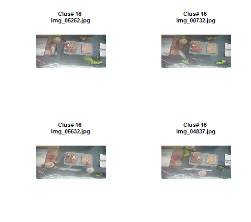
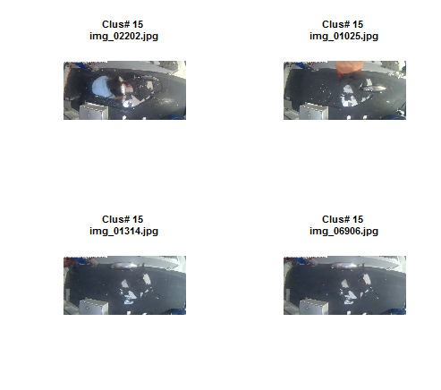
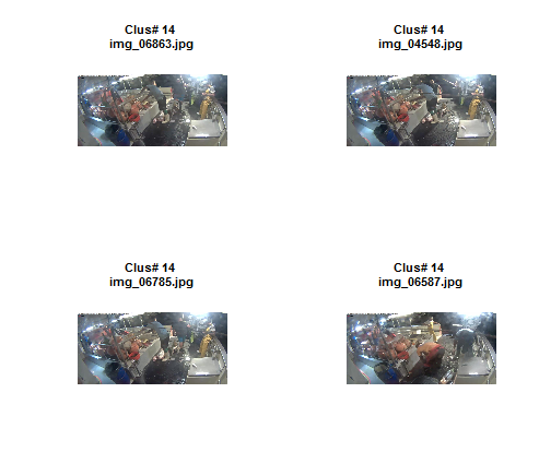
So, its working well. The model is able to club similar images .

Cluster prediction

Now , we can use the model to predict the cluster for all pictures.

The function predict.dbscan(object, data, newdata) [in fpc package] can be used to predict the clusters for the points in newdata. For more details, read the documentation (?predict.dbscan).